Content

Motivation and the binary classification goal

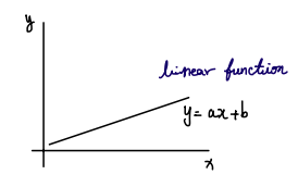
We are all familiar with a linear function. In linear regression, we model the relationship between input $\textcolor{#38bdf8}{x}$ and target $\textcolor{#fb7185}{y}$ with a linear function such as $\textcolor{#fb7185}{y} = a\textcolor{#38bdf8}{x} + \textcolor{#c084fc}{b}$. When we choose linear regression, we are assuming a linear relationship between the data and the outcome we want to predict.

Even with little background, a plot of a linear function already tells you what kind of questions linear regression can answer. The predicted outcome is continuous and can take on any value along the line.

So what do we do if the relationship we want to model is not linear. More specifically, what if the outcome we want to predict only takes two values, 0 and 1.

If the outcome only takes two values, then the outcomes naturally fall into two camps. This is a binary classification problem.

In linear regression, we can plug $\textcolor{#38bdf8}{x}$ into a linear equation and get a continuous prediction. For binary classification, we want a function that produces a value we can interpret as a class and, ideally, as a probability.

There is a standard choice. We use the logistic function, also called the sigmoid.

Setup and notation

We will use the following conventions throughout:

• $\textcolor{#38bdf8}{x}_i \in \mathbb{R}^{d \times 1}$: feature vector for sample $i$
• $\textcolor{#fb7185}{y}_i \in {0,1}$: binary label for sample $i$
• $\textcolor{#93c5fd}{X} \in \mathbb{R}^{n \times d}$: design matrix, where row $i$ is $\textcolor{#38bdf8}{x}_i^\top$
• $\textcolor{#4ade80}{w} \in \mathbb{R}^{d \times 1}$: weight vector, $\textcolor{#c084fc}{b} \in \mathbb{R}$: bias (intercept)
• $\textcolor{#fbbf24}{z} \in \mathbb{R}^{n \times 1}$: score vector, $\textcolor{#2dd4bf}{p} \in (0,1)^{n \times 1}$: predicted probabilities
• $\textcolor{#94a3b8}{\mathbf{1}}_n \in \mathbb{R}^{n \times 1}$: all ones vector

The sigmoid and probability interpretation

Visualization

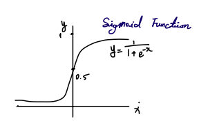
Before worrying about the formula, look at the shape. The curve stays near 0 on the left and near 1 on the right, with a smooth transition in the middle. That already matches what we want for binary classification.

There is another key benefit. The output is always between 0 and 1. That is the range of a probability, so we can interpret the output as the probability of class 1 instead of only making a hard 0 or 1 decision.

Definition

The logistic function maps a scalar $\textcolor{#fbbf24}{z} \in \mathbb{R}$ to a value strictly between 0 and 1:

\[\sigma(\textcolor{#fbbf24}{z}) = \frac{1}{1 + \exp(-\textcolor{#fbbf24}{z})}.\]

For any finite $\textcolor{#fbbf24}{z}$, $\sigma(\textcolor{#fbbf24}{z})\in(0,1)$. It only approaches 0 or 1 in the limits $\textcolor{#fbbf24}{z}\to-\infty$ and $\textcolor{#fbbf24}{z}\to+\infty$.

At this point you might think we can input a sample $\textcolor{#38bdf8}{x}$ into $\sigma$ and get a probability out. Not quite. The sigmoid takes a scalar input $\textcolor{#fbbf24}{z}$, not a feature vector $\textcolor{#38bdf8}{x}$. That is why we introduce a score $\textcolor{#fbbf24}{z}$. The score compresses a multivariate feature vector into a single real number.

We started with a simple goal: predict an outcome $\textcolor{#fb7185}{y}$ from data $\textcolor{#38bdf8}{x}$, where $\textcolor{#fb7185}{y}$ is binary. The sigmoid helps because it maps a real number to a value we can interpret as a probability. The missing piece is how to turn a feature vector into the scalar score that the sigmoid expects.

• The output is always between 0 and 1, which matches the range of a probability.
• Logistic regression is used when we want probabilities for classification.
• It takes a scalar input and outputs a scalar that we interpret as $P(\textcolor{#fb7185}{y}=1 \mid \textcolor{#38bdf8}{x})$.
• The goal is to model the conditional probability of a class given the input.

In the binary case, we usually write

\[\textcolor{#2dd4bf}{p}_i = P(\textcolor{#fb7185}{y}_i = 1 \mid \textcolor{#38bdf8}{x}_i), \qquad 1 - \textcolor{#2dd4bf}{p}_i = P(\textcolor{#fb7185}{y}_i = 0 \mid \textcolor{#38bdf8}{x}_i).\]

Bridge: From probability to a decision

Logistic regression gives probabilities. To turn probabilities into predicted labels, we choose a threshold $\textcolor{#f472b6}{\tau}$ and predict class 1 when the probability is large enough: \(\hat{\textcolor{#fb7185}{y}}_i = \textcolor{#94a3b8}{\mathbf{1}}[\textcolor{#2dd4bf}{p}_i \ge \textcolor{#f472b6}{\tau}].\)

A common default is $\textcolor{#f472b6}{\tau} = 0.5$, but it is often adjusted when classes are imbalanced or when false positives and false negatives have different costs.

Bridge: What is a logit

One key fact is that the logit is the log odds:

\[\operatorname{logit}(\textcolor{#2dd4bf}{p}) = \log\frac{\textcolor{#2dd4bf}{p}}{1-\textcolor{#2dd4bf}{p}}.\]

In logistic regression, the score $\textcolor{#fbbf24}{z}$ is the logit of the class-1 probability: $\textcolor{#fbbf24}{z} = \operatorname{logit}(\textcolor{#2dd4bf}{p})$.

In many ML contexts, the word logits refers to raw real-valued score(s) before applying sigmoid or softmax (binary: a scalar $\textcolor{#fbbf24}{z}$; multiclass: a vector in $\mathbb{R}^K$).

Pointer: this logit link is the core connection to generalized linear models (GLMs), if you add a deeper dive later.

Bridge: Softmax as the multiclass sigmoid

This section is meant for pattern recognition and terminology alignment.

Sigmoid is perfect for binary classification. Many real problems involve more than two classes. Softmax extends the same idea to handle $K$ classes.

Definition

For a vector of scores for one sample $\textcolor{#fbbf24}{z} = [\textcolor{#fbbf24}{z}_1, \textcolor{#fbbf24}{z}_2, \ldots, \textcolor{#fbbf24}{z}_K]$, softmax converts them into a probability distribution:

\[\text{softmax}(\textcolor{#fbbf24}{z})_j = \frac{\exp(\textcolor{#fbbf24}{z}_j)}{\sum_{k=1}^K \exp(\textcolor{#fbbf24}{z}_k)}.\]

In binary logistic regression, we summarize a datapoint with one scalar score. In multiclass classification, we summarize a datapoint with $K$ scores and softmax maps them into $K$ probabilities.

Key properties

• Outputs sum to 1: $\sum_{j=1}^K \text{softmax}(\textcolor{#fbbf24}{z})_j = 1$
• Each output is between 0 and 1
• Differentiable, so we can use gradient based optimization

Connection to the logistic function

When $K = 2$, softmax reduces to sigmoid. Softmax is invariant to adding the same constant to all logits, so we can set logits to $[0, \textcolor{#fbbf24}{z}]$ without loss of generality. Then

\[\text{softmax}([0,\textcolor{#fbbf24}{z}])_1 = \frac{\exp(\textcolor{#fbbf24}{z})}{\exp(0)+\exp(\textcolor{#fbbf24}{z})} = \frac{1}{1+\exp(-\textcolor{#fbbf24}{z})} = \sigma(\textcolor{#fbbf24}{z}).\] \[\text{softmax}([0,\textcolor{#fbbf24}{z}])_0 = \frac{\exp(0)}{\exp(0)+\exp(\textcolor{#fbbf24}{z})} = 1-\sigma(\textcolor{#fbbf24}{z}) = \sigma(-\textcolor{#fbbf24}{z}).\]

So binary logistic regression is the two class softmax model, written with one scalar logit.

The score $\textcolor{#fbbf24}{z}$ and log odds

We want $\textcolor{#2dd4bf}{p}_i = P(\textcolor{#fb7185}{y}_i=1 \mid \textcolor{#38bdf8}{x}_i)$. The sigmoid can produce that probability, but only if we provide a scalar score $\textcolor{#fbbf24}{z}_i$. So we need a way to compute $\textcolor{#fbbf24}{z}_i$ from a feature vector $\textcolor{#38bdf8}{x}_i$.

The score is computed with a linear function. For a feature vector with $d$ features,

\[\textcolor{#fbbf24}{z}_i = \textcolor{#4ade80}{w}^\top \textcolor{#38bdf8}{x}_i + \textcolor{#c084fc}{b}\] \[\textcolor{#38bdf8}{x}_i \in \mathbb{R}^{d \times 1}, \quad \textcolor{#4ade80}{w} \in \mathbb{R}^{d \times 1}, \quad \textcolor{#c084fc}{b} \in \mathbb{R}.\]

Logistic regression interprets this score as a log odds value. For a probability $\textcolor{#2dd4bf}{p}$ of class 1, the log odds is

\[\log\text{-odds} = \log\left(\frac{\textcolor{#2dd4bf}{p}}{1-\textcolor{#2dd4bf}{p}}\right).\]

If $\textcolor{#2dd4bf}{p} = 0.5$, then log odds $= 0$.
If $\textcolor{#2dd4bf}{p} > 0.5$, then log odds $> 0$.
If $\textcolor{#2dd4bf}{p} < 0.5$, then log odds $< 0$.

So log odds acts like a confidence scale for class 1. Logistic regression sets this confidence scale to be linear in the features:

\[\log\left(\frac{\textcolor{#2dd4bf}{p}_i}{1-\textcolor{#2dd4bf}{p}_i}\right) = \textcolor{#4ade80}{w}^\top \textcolor{#38bdf8}{x}_i + \textcolor{#c084fc}{b}.\]

Then we map the score back into probability space using the sigmoid:

\[\textcolor{#2dd4bf}{p}_i = P(\textcolor{#fb7185}{y}_i = 1 \mid \textcolor{#38bdf8}{x}_i) = \sigma(\textcolor{#fbbf24}{z}_i).\]

The full model in matrix form

For $n$ samples, stack the features into a data matrix $\textcolor{#93c5fd}{X}$ and collect scores into a vector $\textcolor{#fbbf24}{z}$:

\[\textcolor{#fbbf24}{z} = \textcolor{#93c5fd}{X}\textcolor{#4ade80}{w} + \textcolor{#c084fc}{b}\textcolor{#94a3b8}{\mathbf{1}}_n, \qquad \textcolor{#2dd4bf}{p} = \sigma(\textcolor{#fbbf24}{z}).\] \[\textcolor{#93c5fd}{X} \in \mathbb{R}^{n \times d},\; \textcolor{#4ade80}{w} \in \mathbb{R}^{d \times 1},\; \textcolor{#c084fc}{b} \in \mathbb{R},\; \textcolor{#fbbf24}{z} \in \mathbb{R}^{n \times 1},\; \textcolor{#fb7185}{y} \in \{0,1\}^{n \times 1},\; \textcolor{#2dd4bf}{p} \in (0,1)^{n \times 1}.\]

Bridge: Wrapping bias into the input matrix

This is a small algebraic trick that removes the separate bias term.

Add a constant feature as the first column of the data matrix: \(\tilde{\textcolor{#93c5fd}{X}} = \begin{bmatrix}\textcolor{#94a3b8}{\mathbf{1}}_n & \textcolor{#93c5fd}{X}\end{bmatrix}\in\mathbb{R}^{n\times(d+1)}.\)

Stack the bias into the weight vector: \(\tilde{\textcolor{#4ade80}{w}}=\begin{bmatrix}\textcolor{#c084fc}{b}\\ \textcolor{#4ade80}{w}\end{bmatrix}\in\mathbb{R}^{(d+1)\times 1}.\)

Then the scores are: \(\textcolor{#fbbf24}{z}=\tilde{\textcolor{#93c5fd}{X}}\tilde{\textcolor{#4ade80}{w}}.\)

Likelihood and binary cross entropy loss

To optimize any model, we need an objective. For logistic regression, we want predicted probabilities that match the observed labels.

Let $\textcolor{#fb7185}{y}_i \in {0,1}$ and $\textcolor{#2dd4bf}{p}_i = P(\textcolor{#fb7185}{y}_i = 1 \mid \textcolor{#38bdf8}{x}_i)$. Then

\[P(\textcolor{#fb7185}{y}_i = 1 \mid \textcolor{#38bdf8}{x}_i) = \textcolor{#2dd4bf}{p}_i, \qquad P(\textcolor{#fb7185}{y}_i = 0 \mid \textcolor{#38bdf8}{x}_i) = 1 - \textcolor{#2dd4bf}{p}_i.\]

This can be written as a Bernoulli likelihood, which measures how likely the model is to assign the observed label:

\[P(\textcolor{#fb7185}{y}_i \mid \textcolor{#38bdf8}{x}_i) = \textcolor{#2dd4bf}{p}_i^{\textcolor{#fb7185}{y}_i} (1-\textcolor{#2dd4bf}{p}_i)^{1-\textcolor{#fb7185}{y}_i}.\]

We want $P(\textcolor{#fb7185}{y}_i \mid \textcolor{#38bdf8}{x}_i)$ to be as high as possible. Equivalently, we minimize $-\log P(\textcolor{#fb7185}{y}_i \mid \textcolor{#38bdf8}{x}_i)$. Define the per sample loss:

\[\begin{align*} \ell_i &= -\log P(\textcolor{#fb7185}{y}_i \mid \textcolor{#38bdf8}{x}_i) \\[0.75em] &= -\log \left(\textcolor{#2dd4bf}{p}_i^{\textcolor{#fb7185}{y}_i} (1-\textcolor{#2dd4bf}{p}_i)^{1-\textcolor{#fb7185}{y}_i}\right) \\[0.75em] &= -\left(\textcolor{#fb7185}{y}_i \log (\textcolor{#2dd4bf}{p}_i) + (1-\textcolor{#fb7185}{y}_i)\log(1-\textcolor{#2dd4bf}{p}_i)\right) \\[0.75em] &= -\textcolor{#fb7185}{y}_i \log(\textcolor{#2dd4bf}{p}_i) - (1-\textcolor{#fb7185}{y}_i)\log(1-\textcolor{#2dd4bf}{p}_i). \end{align*}\]

The average loss over $n$ samples is

\[L = \frac{1}{n}\sum_{i=1}^n \ell_i.\]

This is also called binary cross entropy.

Bridge: Measuring entropy as loss

For Bernoulli targets, minimizing the negative log likelihood is the same as minimizing binary cross entropy.

In ML language, entropy is a measure of uncertainty. Cross entropy measures how misaligned the predicted distribution is with the observed labels.

Gradients of the loss

Logistic regression does not have a closed form solution in general, so we usually use an iterative solver such as gradient descent.

Dependency chain

\[\textcolor{#4ade80}{w}, \textcolor{#c084fc}{b} \to \textcolor{#fbbf24}{z}_i = \textcolor{#4ade80}{w}^\top \textcolor{#38bdf8}{x}_i + \textcolor{#c084fc}{b} \to \textcolor{#2dd4bf}{p}_i = \sigma(\textcolor{#fbbf24}{z}_i) \to L.\]

We compute gradients using the chain rule:

\[\frac{\partial L}{\partial \textcolor{#4ade80}{w}} = \sum_{i=1}^n \frac{\partial L}{\partial \textcolor{#fbbf24}{z}_i}\frac{\partial \textcolor{#fbbf24}{z}_i}{\partial \textcolor{#4ade80}{w}}, \qquad \frac{\partial L}{\partial \textcolor{#c084fc}{b}} = \sum_{i=1}^n \frac{\partial L}{\partial \textcolor{#fbbf24}{z}_i}\frac{\partial \textcolor{#fbbf24}{z}_i}{\partial \textcolor{#c084fc}{b}}.\]

Three derivatives

From $\textcolor{#fbbf24}{z}_i = \textcolor{#4ade80}{w}^\top \textcolor{#38bdf8}{x}_i + \textcolor{#c084fc}{b}$,

\[\frac{\partial \textcolor{#fbbf24}{z}_i}{\partial \textcolor{#4ade80}{w}} = \textcolor{#38bdf8}{x}_i, \qquad \frac{\partial \textcolor{#fbbf24}{z}_i}{\partial \textcolor{#c084fc}{b}} = 1.\]

Since $\textcolor{#2dd4bf}{p}_i = \sigma(\textcolor{#fbbf24}{z}_i)$,

\[\frac{\partial \textcolor{#2dd4bf}{p}_i}{\partial \textcolor{#fbbf24}{z}_i} = \textcolor{#2dd4bf}{p}_i(1-\textcolor{#2dd4bf}{p}_i).\]

Recall

\[\ell_i = -\left(\textcolor{#fb7185}{y}_i \log(\textcolor{#2dd4bf}{p}_i) + (1-\textcolor{#fb7185}{y}_i)\log(1-\textcolor{#2dd4bf}{p}_i)\right).\]

Then

\[\frac{\partial \ell_i}{\partial \textcolor{#2dd4bf}{p}_i} = \frac{1-\textcolor{#fb7185}{y}_i}{1-\textcolor{#2dd4bf}{p}_i} - \frac{\textcolor{#fb7185}{y}_i}{\textcolor{#2dd4bf}{p}_i}.\]

Since $L = \frac{1}{n}\sum_{i=1}^n \ell_i$, we have

\[\frac{\partial L}{\partial \textcolor{#2dd4bf}{p}_i} = \frac{1}{n}\frac{\partial \ell_i}{\partial \textcolor{#2dd4bf}{p}_i}.\]

Collapse to $\textcolor{#2dd4bf}{p}_i - \textcolor{#fb7185}{y}_i$

A standard simplification gives

\[\frac{\partial \ell_i}{\partial \textcolor{#fbbf24}{z}_i} = \textcolor{#2dd4bf}{p}_i - \textcolor{#fb7185}{y}_i.\]

Therefore

\[\frac{\partial L}{\partial \textcolor{#fbbf24}{z}_i} = \frac{1}{n}(\textcolor{#2dd4bf}{p}_i - \textcolor{#fb7185}{y}_i).\]

Final vectorized gradients

Combine the pieces:

\[\nabla_w L = \frac{1}{n}\sum_{i=1}^n (\textcolor{#2dd4bf}{p}_i - \textcolor{#fb7185}{y}_i)\textcolor{#38bdf8}{x}_i, \qquad \frac{\partial L}{\partial \textcolor{#c084fc}{b}} = \frac{1}{n}\sum_{i=1}^n (\textcolor{#2dd4bf}{p}_i - \textcolor{#fb7185}{y}_i).\]

In matrix form,

\[\nabla_w L = \frac{1}{n}\textcolor{#93c5fd}{X}^\top(\textcolor{#2dd4bf}{p}-\textcolor{#fb7185}{y}), \qquad \frac{\partial L}{\partial \textcolor{#c084fc}{b}} = \frac{1}{n}\textcolor{#94a3b8}{\mathbf{1}}_n^\top(\textcolor{#2dd4bf}{p}-\textcolor{#fb7185}{y}).\]

Gradient descent updates

The gradients tell us the local slope of the loss with respect to the parameters. Gradient descent updates the parameters by moving in the negative gradient direction.

With learning rate $\textcolor{#f472b6}{\eta} > 0$, the updates are:

\[\textcolor{#4ade80}{w} \leftarrow \textcolor{#4ade80}{w} - \textcolor{#f472b6}{\eta} \cdot \frac{1}{n}\textcolor{#93c5fd}{X}^\top(\textcolor{#2dd4bf}{p}-\textcolor{#fb7185}{y}), \qquad \textcolor{#c084fc}{b} \leftarrow \textcolor{#c084fc}{b} - \textcolor{#f472b6}{\eta} \cdot \frac{1}{n}\sum_{i=1}^n (\textcolor{#2dd4bf}{p}_i - \textcolor{#fb7185}{y}_i).\]