Content
- Computation and memory
- Finding the K nearest neighbors
- Optional bridges
- Different ways to explore all datapoints
- Distance metrics
- Optional bridges
- Weighted KNN
Nearest = Most Similar?
Let’s assume the following situation. We work at a gardening store and have access to the purchase history of residents in a city, together with their addresses. Now a new resident moves into the city and we want to recommend products to them. The difficult part is that we know almost nothing about this person except where they live.
A natural guess is that nearby residents may have similar gardening needs. If many close neighbors buy products for a hill garden, then the new resident may also have a hill garden and may need similar tools or supplies.
This is the core assumption behind K-nearest neighbors. Points that are close in the feature space are treated as more similar. Once we accept that assumption, prediction becomes simple. To classify a new datapoint, we look at the labels of the nearby training datapoints and let them vote.
Of course, this only works if the feature representation makes distance meaningful. If two datapoints are close according to the chosen features and metric, they should also be similar for the prediction task we care about. If that geometry is poor, then KNN will also perform poorly.
Setup and notation
We will use the following conventions throughout:
- $\textcolor{#38bdf8}{X} \in \mathbb{R}^{n \times d}$: training data matrix with $n$ datapoints and $d$ features
- $\textcolor{#38bdf8}{x}_i \in \mathbb{R}^{d}$: the $i$th training datapoint, stored as the $i$th row of $\textcolor{#38bdf8}{X}$
- $\textcolor{#fb7185}{y} \in {1, …, C}^{n}$: vector of training labels
- $\textcolor{#fb7185}{y}_i \in {1, …, C}$: label of the $i$th training datapoint
- $\textcolor{#c084fc}{x}_\ast \in \mathbb{R}^{d}$: test datapoint
- $\textcolor{#93c5fd}{K} \in {1, …, n}$: number of neighbors used in the vote
So each training example is a pair $(\textcolor{#38bdf8}{x}_i,\textcolor{#fb7185}{y}_i)$ for $i=1,\dots,n$.
The K-Nearest-Neighbor model
The KNN model is simple and intuitive. Given an unseen datapoint $\textcolor{#c084fc}{x}_\ast$, the model finds the $\textcolor{#93c5fd}{K}$ closest training datapoints and predicts the majority class among those neighbors.
There is no parametric model to fit, no weight vector to optimize, and no explicit training objective in the usual sense. The rule is entirely local. The prediction at $\textcolor{#c084fc}{x}_\ast$ depends only on the nearby training samples.
This also means that the decision boundary of KNN is determined directly by the geometry of the training data. If the local neighborhood around $\textcolor{#c084fc}{x}_\ast$ is mixed across classes, then the prediction may be unstable. If the neighborhood is clean and well separated, then the prediction is usually more reliable.
Computation and memory
KNN is an example of a lazy learning model. Unlike many other models, KNN does not build a compact parametric representation during training. In the most basic version, the training stage is almost trivial: we simply store the training dataset and the labels.
This creates a very different trade-off from models such as linear regression, logistic regression, or neural networks.
In a non-lazy model, we usually spend computation during training in order to learn a set of parameters. After training, inference is often cheap because prediction only requires evaluating the learned model.
In a lazy model such as KNN, the opposite happens. Training is cheap because we do not solve an optimization problem, but prediction is expensive because every new test datapoint must be compared against the stored training set.
For brute-force KNN, one query requires computing $n$ distances in a $d$-dimensional space, so the basic inference cost is on the order of $O(nd)$. The memory cost is also significant because we must keep the full training dataset in memory, which is on the order of $O(nd)$ for the features and $O(n)$ for the labels.
So KNN is simple, but that simplicity is not free. It shifts the cost away from training and toward storage and inference.
Finding the K nearest neighbors
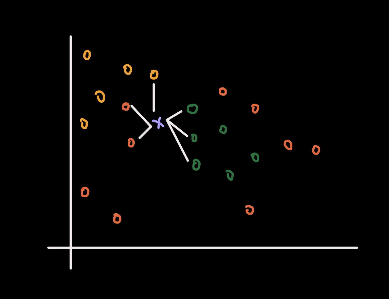
Since there is no conventional training stage, how do we make a prediction for a new datapoint? The answer is simple. We compare the test datapoint $\textcolor{#c084fc}{x}_\ast$ to every training datapoint, compute a distance to each one, sort by closeness, and keep only the $\textcolor{#93c5fd}{K}$ nearest neighbors.
For example, suppose we are doing 3-class classification and set $\textcolor{#93c5fd}{K} = 5$. If among the 5 nearest neighbors, 3 have class label 1, 1 has class label 2, and 1 has class label 3, then we classify the new datapoint as class 1 because it receives the majority vote.
To formalize this inference procedure, let the training set be ${(\textcolor{#38bdf8}{x}i,\textcolor{#fb7185}{y}_i)}{i=1}^n$ with $\textcolor{#fb7185}{y}i \in {1,\dots,C}$ and let the test sample be $\textcolor{#c084fc}{x}\ast \in \mathbb{R}^{d}$.
For each training point, compute the pairwise distance \(d_i=\delta(\textcolor{#c084fc}{x}_\ast,\textcolor{#38bdf8}{x}_i),\quad i=1,\dots,n.\)
Let $\mathcal{N}K(\textcolor{#c084fc}{x}\ast)$ be the index set of the $\textcolor{#93c5fd}{K}$ smallest values among ${d_i}_{i=1}^n$. Then the KNN prediction with majority vote is \(\hat{\textcolor{#fb7185}{y}}(\textcolor{#c084fc}{x}_\ast) = \arg\max_{c\in\{1,\dots,C\}} \sum_{i\in\mathcal{N}_K(\textcolor{#c084fc}{x}_\ast)} \mathbf{1}[\textcolor{#fb7185}{y}_i=c].\)
The indicator function $\mathbf{1}[\textcolor{#fb7185}{y}_i=c]$ equals 1 when neighbor $i$ belongs to class $c$, and 0 otherwise. So the expression simply counts how many of the $\textcolor{#93c5fd}{K}$ nearest neighbors belong to each class, then returns the class with the largest count.
A few practical details matter here.
First, the choice of $\textcolor{#93c5fd}{K}$ controls the bias-variance trade-off. A very small $\textcolor{#93c5fd}{K}$ makes the model highly local and sensitive to noise. A larger $\textcolor{#93c5fd}{K}$ gives a smoother decision rule, but it can oversmooth and ignore local structure.
Second, ties can happen. For example, with an even value of $\textcolor{#93c5fd}{K}$, two classes may receive the same number of votes. In practice, implementations need a tie-breaking rule. Common choices include picking the class with the smaller total neighbor distance, choosing the class with the smaller index, or avoiding ties by using an odd value of $\textcolor{#93c5fd}{K}$ in binary classification.
Third, the notion of closeness is doing almost all of the work. The vote only makes sense once we decide how distance is measured.
Bridge: Different ways to explore all datapoints
The brute-force version of KNN checks the distance from $\textcolor{#c084fc}{x}_\ast$ to every training datapoint, which is simple but expensive when $n$ is large.
This is why search structures such as KD-trees and Ball-trees are useful. They do not change the prediction rule. They only try to avoid unnecessary distance computations by pruning parts of the search space that cannot contain the nearest neighbors.
The key idea is computational, not statistical. The classifier is still KNN. We are only changing how we search for $\mathcal{N}K(\textcolor{#c084fc}{x}\ast)$.
There are also approximate nearest neighbor methods. These methods may return neighbors that are not exactly optimal, but they can be much faster in large datasets or high-dimensional spaces. This trade-off is often worthwhile when exact search becomes too slow.
Define “closest neighbors” and distance metrics.
Everything now depends on the choice of distance metric. Different metrics encode different notions of similarity, so the metric should match the structure of the features.
Minkowski Distance
Minkowski distance is one of the most common choices because it is a family of distance metrics indexed by a parameter $p \ge 1$:
\(d(\textcolor{#c084fc}{x}_\ast,\textcolor{#38bdf8}{x}_i)
=
\left(
\sum_{j=1}^{d}
\left|
\textcolor{#c084fc}{x}_{\ast,j}-\textcolor{#38bdf8}{x}_{i,j}
\right|^p
\right)^{1/p}.\)
Two important special cases are:
- when $p=1$, this becomes Manhattan distance
- when $p=2$, this becomes Euclidean distance
These distances are sensitive to feature scale. If one feature has a much larger numerical range than the others, then that feature can dominate the distance computation and effectively control the neighborhood structure. Because of this, feature scaling is usually essential before applying KNN with Manhattan or Euclidean distance.
Hamming Distance
Hamming distance is often used when the features are binary or one-hot encoded. It counts how many coordinates differ between two vectors:
\(d(\textcolor{#c084fc}{x}_\ast,\textcolor{#38bdf8}{x}_i)
=
\sum_{j=1}^{d}
\mathbf{1}[\textcolor{#c084fc}{x}_{\ast,j}\neq \textcolor{#38bdf8}{x}_{i,j}].\)
So two datapoints are considered close if they match on many coordinates. This is often more appropriate than Euclidean distance when the features are categorical indicators rather than continuous measurements.
Cosine Distance
Cosine distance is useful when direction matters more than magnitude. This often happens in text data, embeddings, or sparse high-dimensional representations.
First define cosine similarity: \(\text{cosine similarity}(\textcolor{#c084fc}{x}_\ast,\textcolor{#38bdf8}{x}_i) = \frac{\textcolor{#c084fc}{x}_\ast^\top \textcolor{#38bdf8}{x}_i} {\|\textcolor{#c084fc}{x}_\ast\| \, \|\textcolor{#38bdf8}{x}_i\|}.\)
A larger cosine similarity means the two vectors point in a more similar direction. To convert this into a distance-like quantity, we use \(d(\textcolor{#c084fc}{x}_\ast,\textcolor{#38bdf8}{x}_i) = 1- \frac{\textcolor{#c084fc}{x}_\ast^\top \textcolor{#38bdf8}{x}_i} {\|\textcolor{#c084fc}{x}_\ast\| \, \|\textcolor{#38bdf8}{x}_i\|}.\)
So cosine distance ignores overall scale and focuses on angular alignment. Two vectors can have very different magnitudes and still be close under cosine distance if they point in nearly the same direction.
The choice of metric is not a minor implementation detail. It determines what the model means by similar, which in turn determines which datapoints are allowed to vote.
Bridge: Weighted KNN
A natural extension of the standard KNN rule is the following. If closer datapoints are more similar to the test datapoint, then it is reasonable to let closer neighbors have more influence on the final vote.
This is the idea behind weighted KNN. Instead of giving each of the $\textcolor{#93c5fd}{K}$ neighbors one equal vote, we assign a nonnegative weight to each neighbor based on its distance to $\textcolor{#c084fc}{x}_\ast$. Smaller distance should correspond to larger weight.
One common choice is inverse-distance weighting: \(w_i=\frac{1}{d_i+\epsilon}, \quad i\in \mathcal{N}_K(\textcolor{#c084fc}{x}_\ast),\) where $\epsilon > 0$ is a very small constant used to avoid division by zero.
The prediction rule becomes \(\hat{\textcolor{#fb7185}{y}}(\textcolor{#c084fc}{x}_\ast) = \arg\max_{c\in\{1,\dots,C\}} \sum_{i\in\mathcal{N}_K(\textcolor{#c084fc}{x}_\ast)} w_i \mathbf{1}[\textcolor{#fb7185}{y}_i=c].\)
So the model is still doing a vote, but now it is a weighted vote. A neighbor that is extremely close to $\textcolor{#c084fc}{x}_\ast$ can matter more than a neighbor that is only barely inside the $\textcolor{#93c5fd}{K}$ nearest set.
This is often useful near class boundaries. Under ordinary KNN, a moderately far group of neighbors can outvote a very close and highly relevant datapoint simply because each vote counts equally. Weighted KNN reduces that problem by letting distance affect influence directly.
If a training point lands exactly on the query point so that $d_i=0$, then weighted KNN places almost all of the mass on that point. Conceptually, this is sensible. If we have already seen the exact same feature vector in the training set, then its label should strongly influence the prediction.
There are other weighting choices as well, such as Gaussian-style weights, but inverse-distance weighting already captures the main idea: not all neighbors inside the $\textcolor{#93c5fd}{K}$ set should necessarily count the same.
Conclusion
K-nearest neighbors is one of the simplest classification models, but it already captures several important ideas in machine learning. The model assumes that nearby datapoints should behave similarly, so prediction reduces to a local vote among the nearest training examples.
That simplicity is what makes KNN easy to understand, but it also makes every design choice matter. The value of $\textcolor{#93c5fd}{K}$ controls how local the rule is. The distance metric determines what counts as similar. The feature representation decides whether that notion of similarity is meaningful at all.
So even though the prediction rule is short, the real behavior of KNN is shaped by geometry. If the features are well scaled and the metric matches the data, KNN can work surprisingly well. If the geometry is poor, then the nearest neighbors may not be relevant neighbors.
This is also why KNN is a useful model to study early. It makes the role of distance, locality, and representation very explicit. There is no hidden optimization and no learned parameter vector that obscures what the model is doing. The classifier is only comparing datapoints, selecting neighbors, and voting.
So the main lesson is simple. KNN works when closeness is a meaningful proxy for similarity. Once that assumption is reasonable, the rest of the method follows naturally.